5. 19-port photonic lantern#
5.1. overview and challenges#
In this example, we will simulate a 19-port photonic lantern with hexagonally packed cores. The two main complexities are: a (perhaps unexpected) eigenvalue crossing; and widespread degeneracy of the modes at the larger end of the lantern. While a straight calculation using the techniques from prior examples will work, such a calculation would require a very fine \(z\)-step resolution and take a long time.
To identify these issues before actually running characterize(), we will first compute the effective index structure of the device, which is often much faster than a blind calculation of the eigenmodes because the effective indices will vary more smoothly than the eigenmodes. This will be done using the function
propagator.compute_neffs()
5.2. computing effective indices#
First, I’ll set the parameters.
wl = 0.8                         # wavelength, um
taper_factor = 12.               # relative scale factor between frontside and backside waveguide geometry
rcore = 1.8/taper_factor         # radius of tapered-down single-mode cores at frontside (small end), um
rclad = 9.0                      # radius of cladding-jacket interface at frontside, um
rjack = 27                       # radius of outer jacket boundary at frontside, um
z_ex = 100000                    # lantern length, um

nclad = 1.444                    # cladding refractive index
ncore = nclad + 8.8e-3           # SM core refractive index
njack = nclad - 5.5e-3           # jacket (low-index capillary) refractive index

rcores = [rcore]*19
ncores = [ncore]*19
Next, we’ll make the lantern. The 19 cores will be placed in a hexagonal array.
from cbeam.waveguide import get_19port_positions
core_pos = get_19port_positions(rclad/2.5)

# mesh params #
core_res = 16
clad_res = 60
jack_res = 30

from cbeam.waveguide import PhotonicLantern
PL19 = PhotonicLantern(core_pos,rcores,rclad,rjack,ncores,nclad,njack,z_ex,taper_factor,core_res,clad_res,jack_res)
Finally, we’ll run compute_neffs(). The syntax is similar to characterize(), and you can save and load files as well. Even though we expect this waveguide to support 19 guided modes, we will solve for the 21 highest effective indices, since there is no guarantee that the 19 highest index modes at the start of the waveguide correspond with the 19 highest index modes at the end of the waveguide. (In practice, you would probably design the waveguide such that there are no crossings in the first place, at least for the modes you care about).
from cbeam.propagator import Propagator

prop = Propagator(wl,PL19,Nmax=21)

# comment/uncomment as necessary
prop.compute_neffs()
# prop.load(tag="19port_neffs")
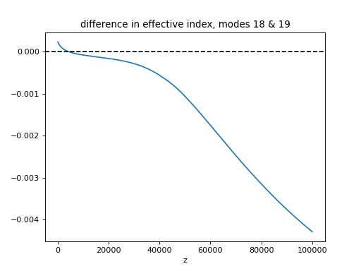
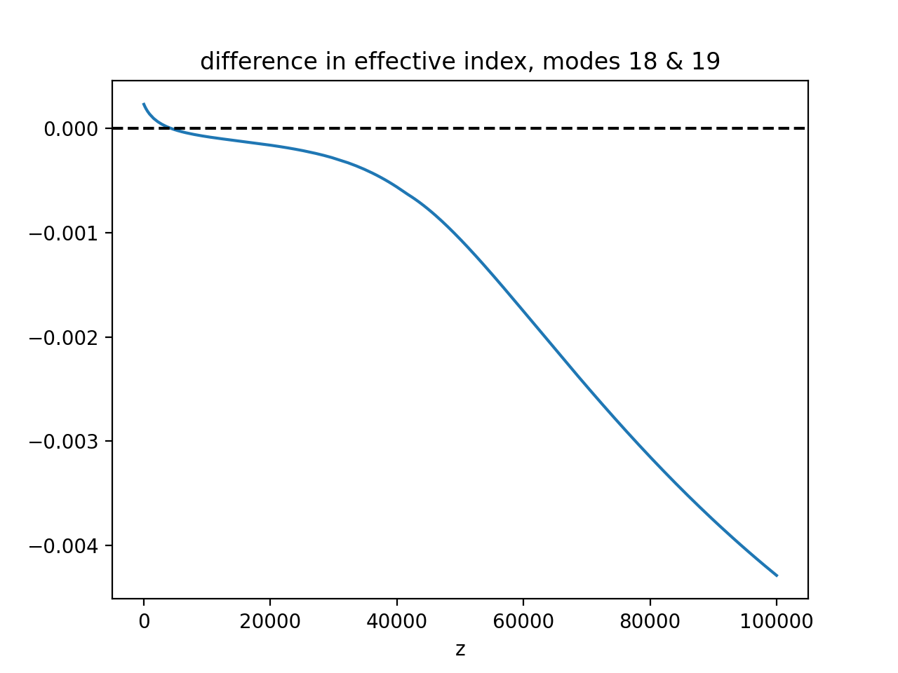
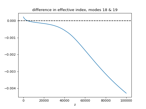
Next, I’ll plot the effective indices, as well as the difference in index between modes 18 and 19, to show that they cross early on.
import matplotlib.pyplot as plt
plt.plot(prop.zs,prop.neffs[:,18]-prop.neffs[:,19])
plt.axhline(y=0,color='k',ls='dashed')
plt.xlabel("z")
plt.title("difference in effective index, modes 18 & 19")
plt.show()
(Source code, png, hires.png, pdf)
prop.plot_neff_diffs()
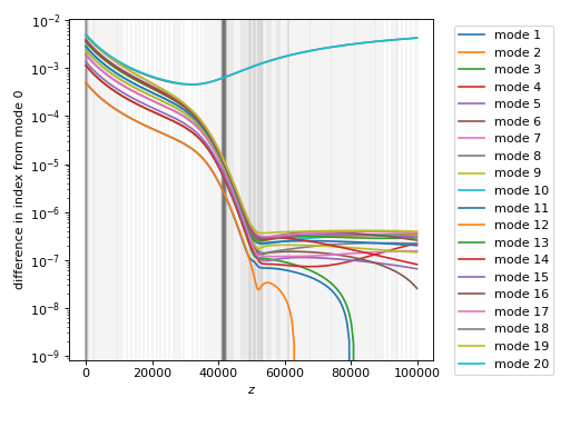
As before, the vertical lines show the \(z\) locations traversed during the computation. The dark band a little after \(z=40\) mm is actually a result of another eigenvalue crossing, this time between a cladding mode and a higher-order mode that was not included in the 21 initial modes.
From the effective index information, we can identify groups of degenerate modes. First, certain mode pairs remain degenerate through the entirety of the waveguide; second, all of the guided eigenmodes become degenerate in the back half of the waveguide. This suggests that the simulation should be done in two or more pieces, each with different specifications for mode degeneracy.
Note
Why does accounting for mode degeneracy need to be done manually? In the past, I tried to manage this automatically, by fixing subspaces of the eigenbasis when the difference in eigenvalues was sufficiently low. However, switching this correction on and off breaks eigenmode differentiability. Situations where a degeneracy is formed and then later broken add even more complexity.
5.3. characterize the front half#
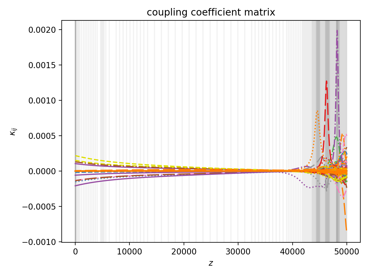
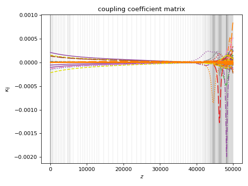
Below is the characterization of the front half of the lantern. I also plot the coupling coefficients. This takes around 6 minutes on my desktop.
# from the previous analysis, we only need to track the top 20 modes
# to ensure that all guided modes are tracked
prop1 = Propagator(wl,PL19,20)

prop1.degen_groups = [[1,2],[3,4],[6,7],[8,9],[10,11],[12,13],[15,16]]

# during characterization, we specify modes we don't care about
# to speed things up. mode 18 becomes a cladding mode, as
# per previous analysis.
prop1.skipped_modes = [18]

tag1 = "19port_0800_front"
prop1.characterize(0,50000,save=True,tag=tag1)
# prop1.load(tag1)

prop1.plot_coupling_coeffs(legend=False)
(Source code, png, hires.png, pdf)
5.4. characterize the back half#
We will make another Propagator object to perform the back half characterization, where all guided modes (i.e. every mode except 18) are assumed degenerate. We also need to ensure this propagator uses the final eigenbasis from earlier, which we can do using Propagator.load_init_conds().
tag2 = "19port_0800_back"
prop2 = Propagator(wl,PL19,20)
prop2.skipped_modes = [18]
# every mode except 18 is degenerate w/ each other
prop2.degen_groups = [[i for i in range(20)]]
del prop2.degen_groups[0][18]
# use the final modes of prop1 as the
# initial modes of prop2
prop2.load_init_conds(prop1)
prop2.characterize(50000,100000,save=True,tag=tag2)
# prop2.load(tag2)
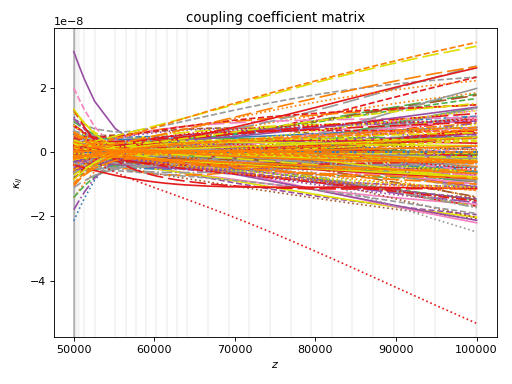
prop2.plot_coupling_coeffs(legend=False)
(Source code, png, hires.png, pdf)
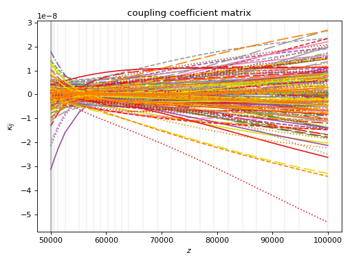
Yeah, it looks like a mess.
Collectively, both characterizations take around 800 seconds on my laptop.
5.5. end-to-end propagation#
We will combine the two propagators using the ChainPropagator class, which lets us to send wavefronts through a list of propagators. Below, I launch the \(LP_{01}\) mode.
from cbeam.propagator import ChainPropagator
prop12 = ChainPropagator([prop1,prop2])
u0 = [0.]*20
# launch LP01
u0[0] = 1.
# propagate as normal
zs,us,uf = prop12.propagate(u0)
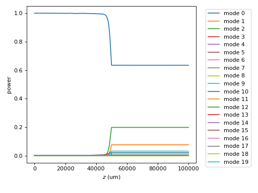
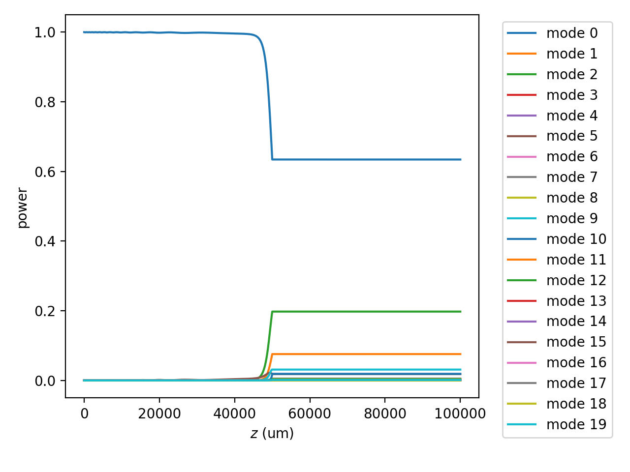
prop12.plot_mode_powers(zs,us)
(Source code, png, hires.png, pdf)

You can see the mode powers are nearly frozen in the back half of the lantern, because the eigenbasis has been fixed (as much as possible) for that portion of the calculation. We can also view fields as usual:
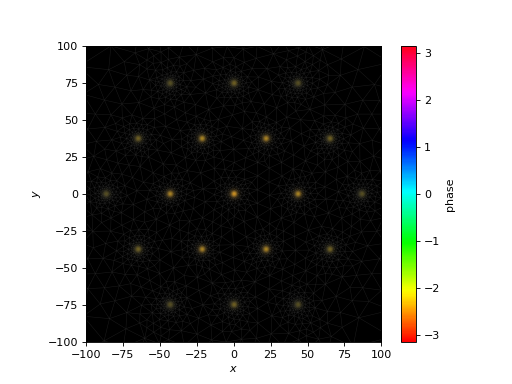
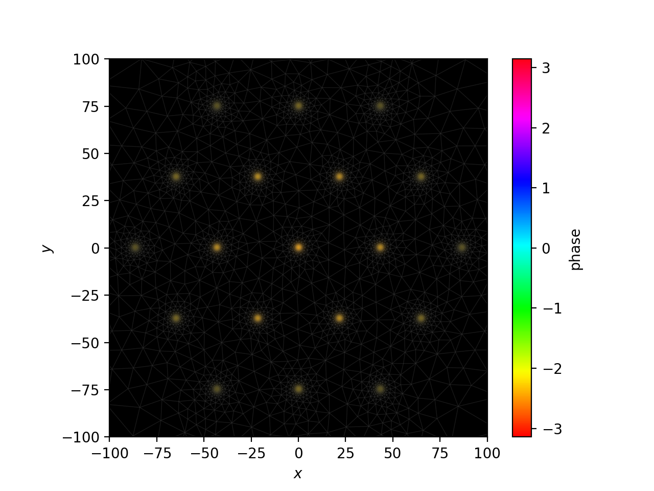
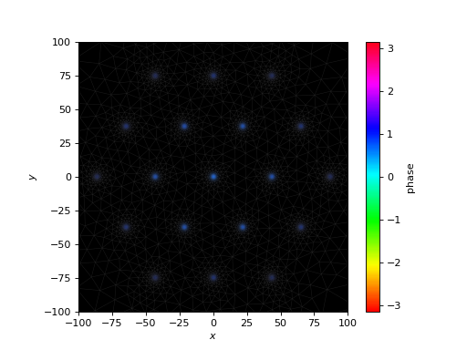
f = prop12.make_field(us[-1],zs[-1])
prop12.plot_cfield(f,zs[-1],res=0.25,show_mesh=True,xlim=(-100,100),ylim=(-100,100))
(Source code, png, hires.png, pdf)
Finally, we can extract the channel powers using
out = prop12.to_channel_basis(uf)
print(np.power(np.abs(out),2))
[0.15452255 0.09629082 0.09613682 0.09645077 0.09615026 0.09584128 0.09597969 0.01385659 0.03039846 0.01383495 0.03037306 0.01381777 0.0303713 0.0138303 0.03044344 0.01383603 0.03046803 0.01379971 0.03046496]
In this example, propagations take a few seconds. For repeat propagations, it is much faster to use a transfer matrix. This can be done with
M = prop12.compute_transfer_matrix()
# and then propagation is ...
uf = np.dot(M,u0)