quickstart

1. overview

cbeam provides the following submodules.

• cbeam.waveguide : used to define waveguides.

• cbeam.propagator : used to define propagation parameters and run propagations.

The typical workflow is to first define a waveguide, and then pass it to a propagator object to characterize the waveguide and then propagate fields through it.

2. waveguide basics

Waveguides in cbeam are defined as classes. There are several pre-defined classes, and users may define their own which inherit from a base Waveguide class. The full documentation is here.

Below are some pre-defined waveguides.

• CircularStepIndexFiber : a straight, circular, step-index optical fiber.

• RectangularStepIndexFiber : a straight, step-index fiber with a rectangular core.

• Dicoupler : 2x2 directional coupler with circular channels.

• Tricoupler : a 3x3 directional coupler with circular channels, in equilateral triangle configuration.

• PhotonicLantern : a linearly tapered photonic lantern, with circular cores, cladding, and jacket.

Waveguide objects have two major functions. First, the Waveguide object is responsible for creating a finite-element mesh, e.g. through

mesh = Waveguide.make_mesh()

This mesh is used to solve for eigenmodes. Second, if waveguide’s cross section varies with distance along the propagation axis, the mesh must be deformed to follow this variation; this is covered more in the Waveguide class. Waveguide objects also have plotting functions to view the mesh and refractive index profile, e.g.

from cbeam import waveguide

# make a waveguide for testing - 6 port photonic lantern
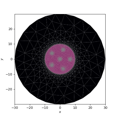
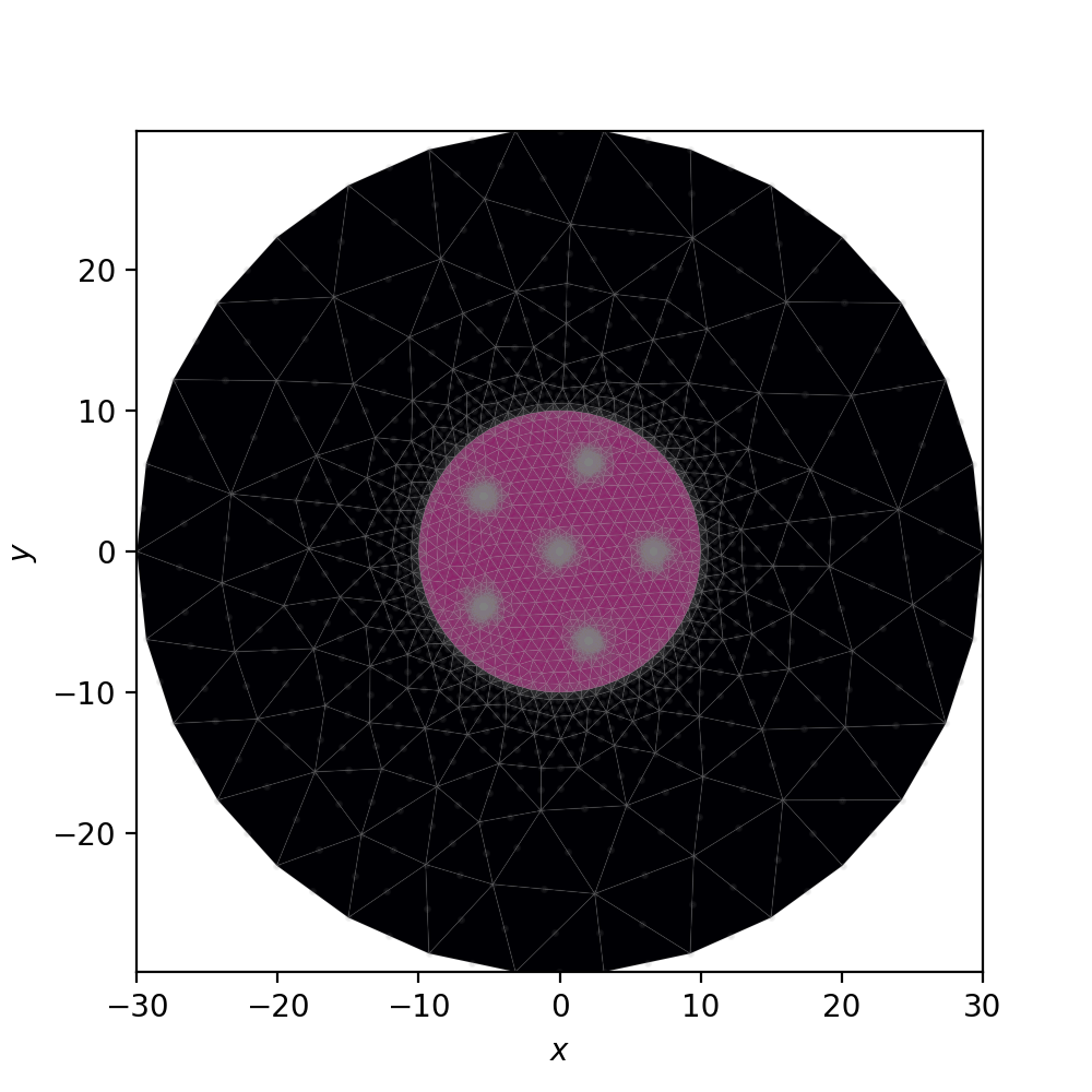
wvg = waveguide.TestPhotonicLantern()
mesh = wvg.make_mesh()

wvg.plot_mesh(mesh=mesh) # can also leave out mesh; a mesh will be auto-generated

(Source code, png, hires.png, pdf)

3. propagator basics

The Propagator class is responsible for computing the necessary properties of the waveguide for coupled-mode propagation, as well as the propagation itself. The full documentation is here.

A Propagator is initialized as

prop = propagator.Propagator(wl, wvg, Nmax)

where the arguments are as follows.

1. wl : the propagation wavelength (in the same spatial unit that the waveguide geometry is defined in)

2. wvg : a Waveguide object

3. Nmax : the number of propagating modes you want to track within the waveguide (modes are ordered by their initial effective index.)

waveguide characterization

Before we can perform optical propagations, we need the following as a function of \(z\) (the longitudinal coordinate of the waveguide) :

1. the instanteous eigenmodes

2. the instanteous eigenvalues

3. the coupling coefficient matrix

To compute these values, we use

prop.characterize(save,tag)

The results are saved to file when save=True; tag is a string that will be added to the filenames. Results are loaded through

prop.load(tag)

For more details, check out advanced usage.

propagation

Once the waveguide has been characterized, we can propagate fields through it. The general syntax is

zs,us,uf = prop.propagate(u0,zi,zf)

where u0 the launch field, expressed in the modal basis of waveguide modes, and zi and zf are the starting and ending \(z\) coordinates. This returns 3 items:

1. zs : an array of \(z\) values selected by the diff eq solver used to solve the coupled-mode equations.

2. us : an array of amplitudes for the eigenmodes at each \(z\) (with most of the complex phase oscillation factored out, as per coupled-mode theory). The first axis corresponds with zs.

3. uf : the final mode amplitudes (with phase oscillation factored in) - these are the actual complex-valued mode amplitudes at zf, evaluated in the basis of the final eigenmodes.

To convert a mode amplitude vector to an electric field (represented as a 2D numpy array), you can use

field = prop.make_field(mode_vector,z)

where mode_vector is an array of mode amplitudes (e.g. any row of u, but not uf) and z is the \(z\) coordinate of the mode vector. You can also generate a plot with plot=True. Otherwise, use the following for complex-valued fields

prop.plot_cfield(field,z)

# or, if you want a lower-fidelity, interactive plot
# where you can change z
prop.plot_wavefront(zs,us)

For plotting waveguide eigenmodes as a function of \(z\), there is a dedicated function.

# plot eigenmode i
Propagator.plot_waveguide_mode(i)

putting it all together

… looks something like this:

from cbeam.propagator import Propagator
from cbeam.waveguide import TestPhotonicLantern

# make the waveguide
wvg = TestPhotonicLantern()

wavelength = 1.55 # um
num_modes = 6 # assuming we're using the 6-port lantern from earlier
tag = "test"

# make the propagator
prop = Propagator(wavelength,wvg,num_modes)

# characterization - comment/uncomment below as needed
# prop.characterize(save=True,tag=tag)
prop.load(tag=tag)

u0 = [1,0,0,0,0,0] # starting mode vector, corresponding to fundamental mode

# this returns the z values, coupled-mode amplitudes, and the output amplitudes
zs,us,uf = prop.propagate(u0)

(Source code)

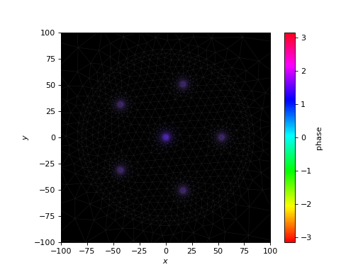
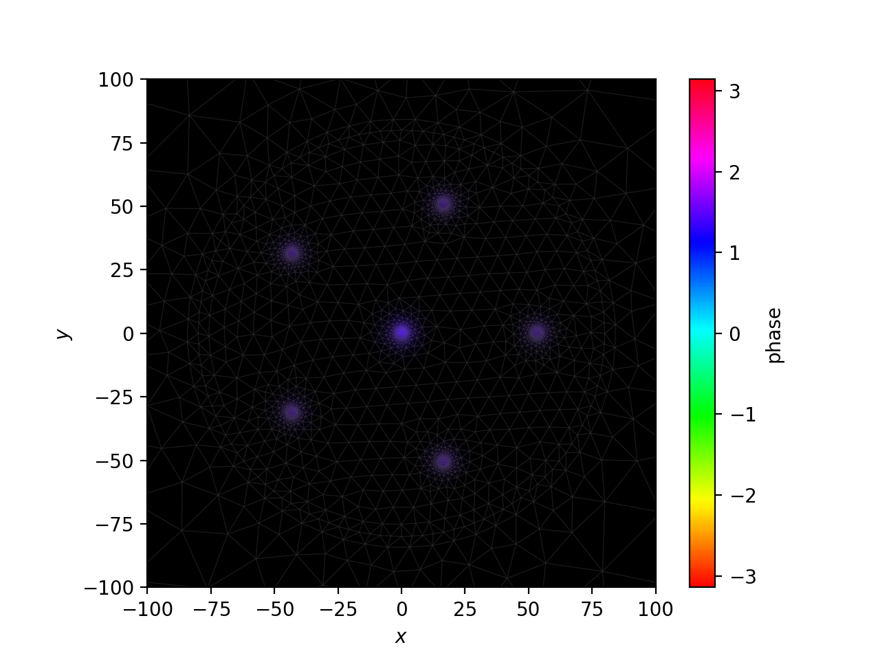
We’ll plot the final field below.

# get the fields and plot
output_field = prop.make_field(us[-1],zs[-1])

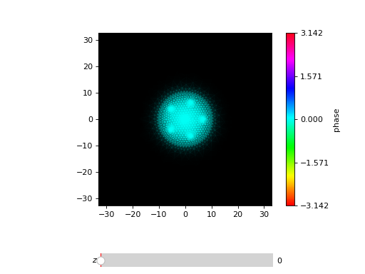
prop.plot_cfield(output_field,z=zs[-1],show_mesh=True,xlim=(-100,100),ylim=(-100,100),res=0.5)

(Source code, png, hires.png, pdf)

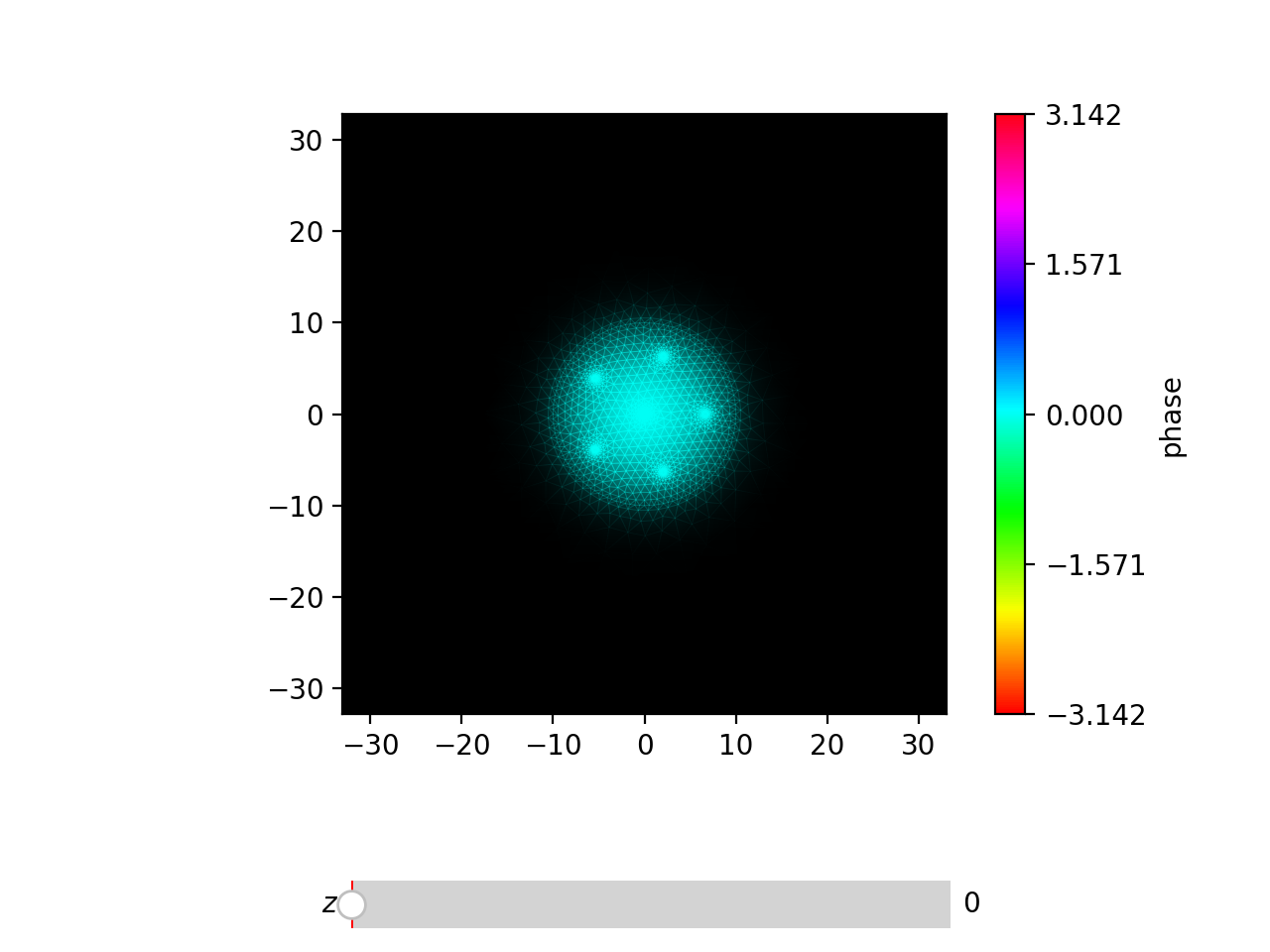
Alternately, we can see how the wavefront propagates through the waveguide using an interactive plot.

prop.plot_wavefront(zs,us)

(Source code, png, hires.png, pdf)

The mesh lines are also shown (areas where there are a lot of mesh lines may appear brighter). The slider sadly doesn’t work inside the webpage.

4. tips

• Keep track of how many points are in your mesh. Most testing so far has been done on meshes with 1,000 to around 15,000 points. You use more points but memory and storage may become an issue.

• Be aware of potential sources of discretization error when making meshes for waveguides (e.g. representing circles as polygons).

• You can control the adaptive stepping accuracy with Propagator.z_acc.

Now you are ready to look at the examples!