4. multimode interference coupler

Note

This example is for a weakly guided multimode interference (MMI) coupler, which is a little unusual: typical MMI couplers use strong index contrasts and have highly confined modes, which I think give better performance.

A multimode interference (MMI) coupler can be constructed using a series of \(M\) “access” waveguides and \(N\) output waveguides which are connected in the middle by a larger, multimoded slab waveguide. Under certain design parameters, an MMI coupler acts as an \(M\times N\) beam recombiner. Such devices leverage the “self-imaging” property of the central slab waveguide. This section presents a partial simulation of a \(1 \times 3\) MMI coupler, and also shows how electric fields from one waveguide mesh can be transferred to another.

4.1. waveguide setup

Below, I lay out some parameters. Both the access waveguide and center waveguide are modeled as rectangular core step-index fibers, which we will model separately.

from cbeam.waveguide import RectangularStepIndexFiber

mmi_width = 60. # width of the slab's core
mmi_height = 6. # height of the slab's core

access_width = 6. # same for the access waveguide
access_height = 6.

wl = 1.55   # wavelength

ncore = 1.445   # core index
nclad = 1.44    # cladding index

access = RectangularStepIndexFiber(access_width,access_height,access_height*6,access_width*6,ncore,nclad,1.,5.)
mmi = RectangularStepIndexFiber(mmi_width,mmi_height,mmi_width*3,mmi_height*6,ncore,nclad,1.,5.)

(Source code)

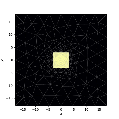
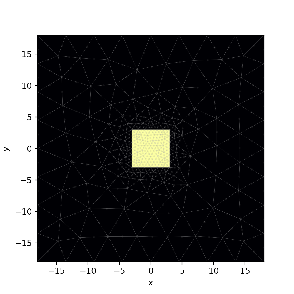
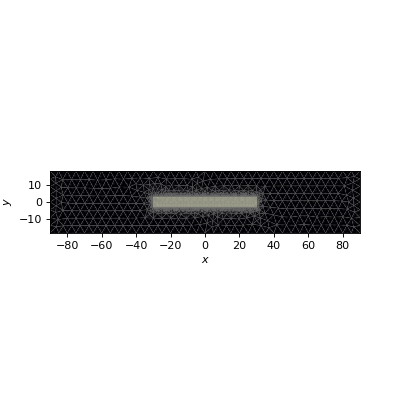
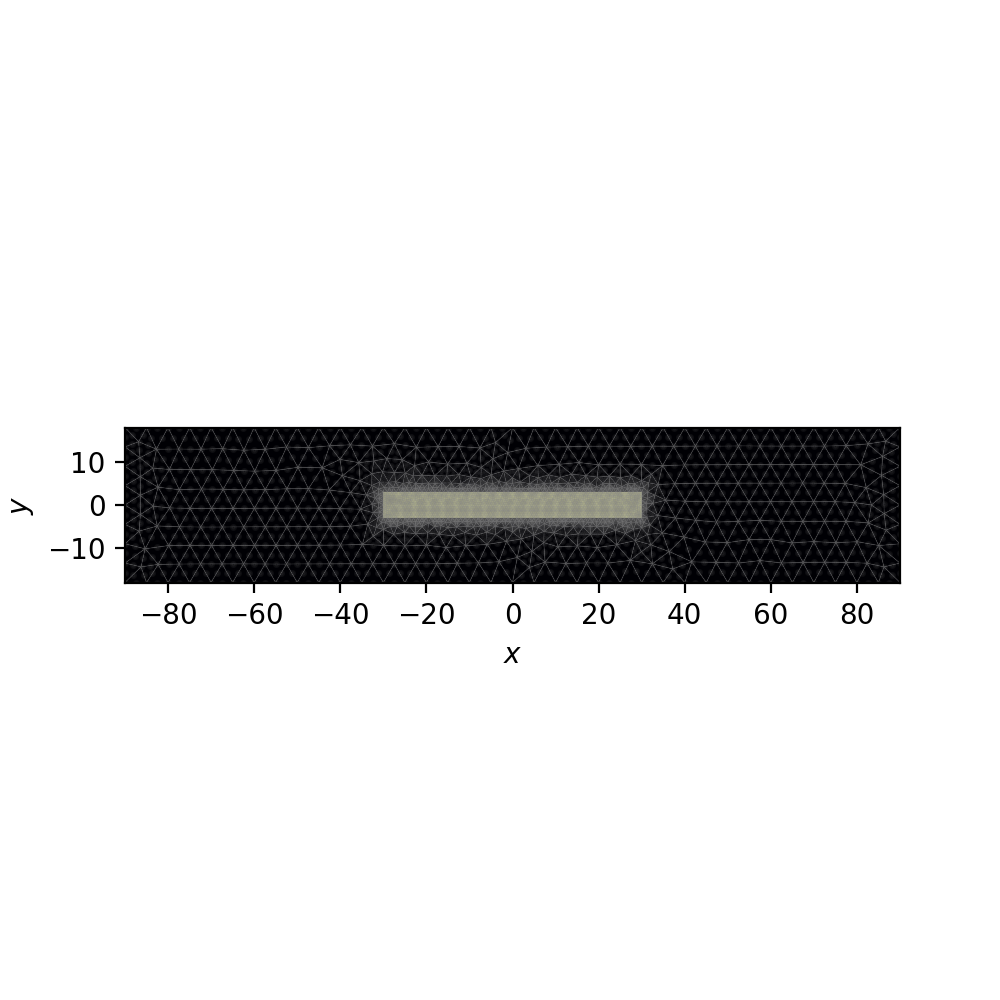
Let’s plot the meshes and refractive indices for both the access waveguide and central MMI section.

access.plot_mesh()
mmi.plot_mesh()

(Source code)

(png, hires.png, pdf)

(png, hires.png, pdf)

4.2. access waveguide

In our \(1\times 3\) MMI coupler design, the access waveguide is centrally connected to one end of the central slab. Thus, to determine our launch field in the central slab, we will first do a mode solve of the access waveguide.

from cbeam.propagator import Propagator

access_prop = Propagator(wl,access,Nmax=1)
ac_neffs,ac_modes = access_prop.solve_at(0)

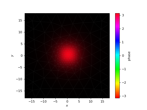
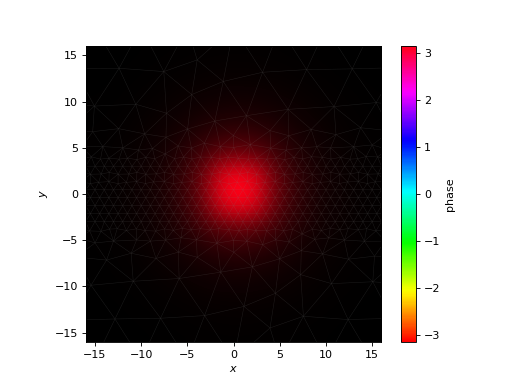
access_prop.plot_cfield(ac_modes[0],show_mesh=True)

(Source code, png, hires.png, pdf)

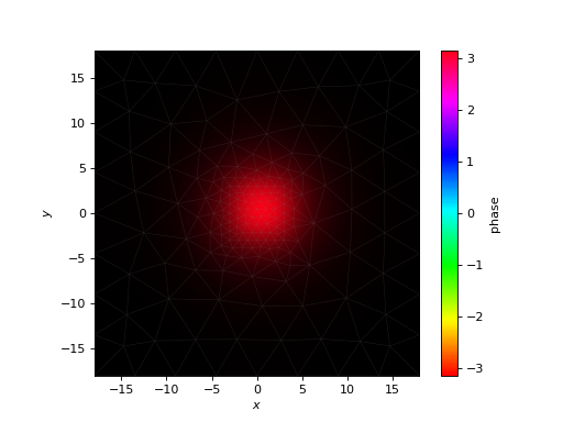
The above is the field we’ll launch into the slab.

4.3. MMI characterization

Next, we’ll compute the propagation characteristics of the slab. Mathematically, this is super simple because the waveguide doesn’t change with \(z\), and all the coupling coefficients are 0. But the syntax is the same:

# last time i checked there are 8 guided modes
# you can double check though.
mmi_prop = Propagator(wl,mmi,Nmax=8)
mmi_prop.characterize()

(Source code)

4.4. moving between meshes

Next, we will “transfer” our launch field, which is defined on the access waveguide mesh, to the mesh of the slab waveguide section. To do this, we will use cbeam.FEval.resample().

from cbeam import FEval

# resample takes: input field, input mesh, output mesh
launch_field = FEval.resample(ac_modes[0],access_prop.mesh,mmi_prop.mesh)

# we'll plot to make sure it looks good
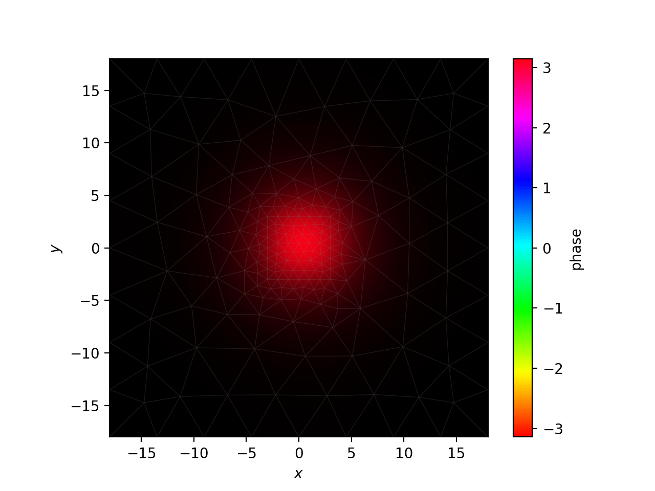
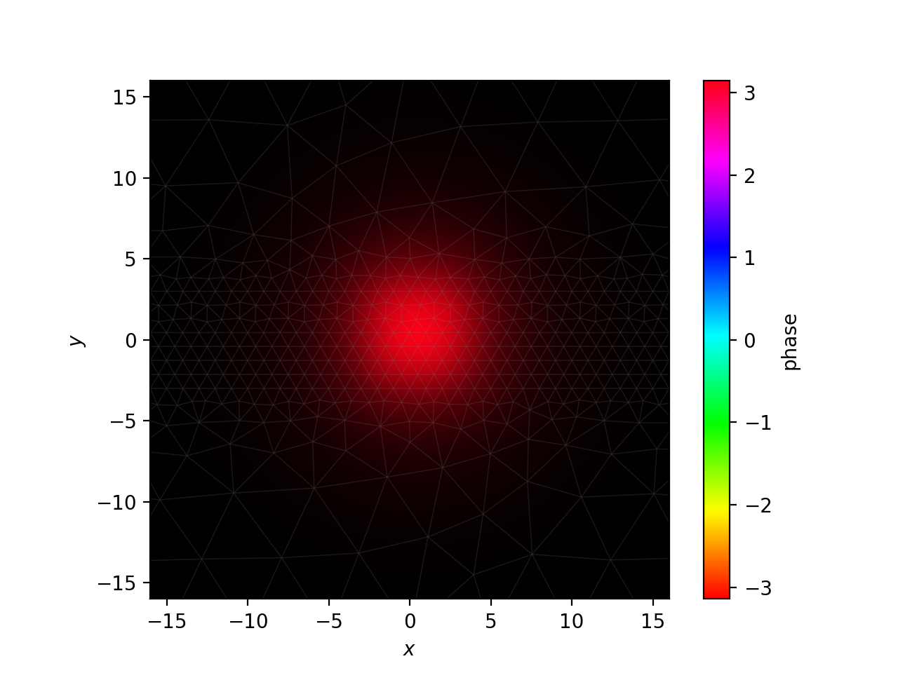
mmi_prop.plot_cfield(launch_field,xlim=(-16,16),ylim=(-16,16),show_mesh=True)

(Source code, png, hires.png, pdf)

The last step before propagation is to convert our field into a mode amplitude vector, which is done using Propagator.make_mode_vector():

launch_modes = mmi_prop.make_mode_vector(launch_field)
print(launch_modes)

(Source code)

[6.59948619e-01 3.83775210e-05 -5.32959493e-01 2.76286527e-05 -3.80385142e-01 3.48737666e-05 2.56268483e-01 3.06148543e-05]

The total power of the above turns out to be less than 1, indicating that some power will be lost to radiative modes. These losses can be mitigated by tapering the access waveguide (like the tapered box fiber in fiber mode solving), though this is outside the scope of the example.

4.5. propagation

One nuance in this example is that we don’t need to formally propagate, since all the coupling coefficients are 0. The power in each mode is preserved; the only thing we need to do is apply the phase evolution for each mode. This means we can directly get the propagated fields with Propagator.make_field(). I will plot the field at the expected \(z\) coordinate for a three-fold self image.

betas = mmi_prop.neffs[0] * 2 * np.pi / wl
L = np.pi/(betas[0]-betas[1])

f = mmi_prop.make_field(launch_modes,z=L/4,apply_phase=True)

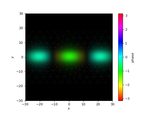
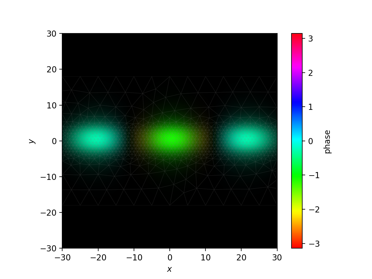
mmi_prop.plot_cfield(f,xlim=(-30,30),ylim=(-30,30),show_mesh=True)

# you could also do
# zs,us,uf = mmi_prop.propagate(launch_mvec,0,L/4)
# f = prop.make_field(uf,apply_phase=False)

(Source code, png, hires.png, pdf)

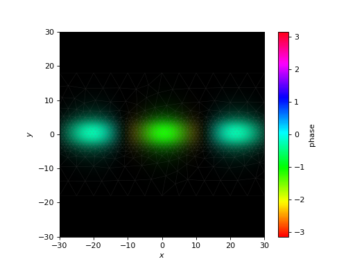
We get three images of the launch field, as expected. From this point, we could construct a 3-channel output waveguide to couple this field into. Splitting the beam further seems difficult with this design, likely because it is only weakly guiding.

For reference, I used the following formulas to compute the required self-imaging distance. Denote \(\beta_j\) the propagation constant of mode \(j\), which is related to \(n_j\), the effective index of mode \(j\), by \(\beta_j=k n_j\) ; \(k\) is the free-space wavenumber. Define the beat length between the two lowest-order modes as

\[L_\pi \equiv \dfrac{\pi}{\beta_0-\beta_1}.\]

When launching a symmetric field, the first \(N\)-fold self-image will be formed at a distance

\[L = \dfrac{3 L_\pi}{4N}.\]

References

1. 12. 2. Soldano and E. C. M. Pennings, “Optical multi-mode interference devices based on self-imaging: principles and applications,” in Journal of Lightwave Technology, vol. 13, no. 4, pp. 615-627, April 1995, doi: 10.1109/50.372474.