1. fiber mode solving

1.1. straight circular fiber

On this page, we’ll use cbeam to solve for the modes of some optical fibers. This will also show how more complicated waveguides can be defined. First, let’s make a circular fiber - from “scratch”. We’ll use waveguide.Pipe to make a cladding cylinder and a core cylinder.

from cbeam import waveguide
rcore,rclad = 10,30 # units are in whatever we choose for wavelength later, which will be um.
ncore,nclad = 1.445,1.44
res = 30 # resolution
core = waveguide.Pipe(ncore,"core",res,rcore)
clad = waveguide.Pipe(nclad,"clad",3*res,rclad)

(Source code)

core and clad are building blocks. We combine them as a Waveguide:

fiber = waveguide.Waveguide([clad,core])
fiber.z_invariant = True # tell cbeam that this waveguide does not change with z

(Source code)

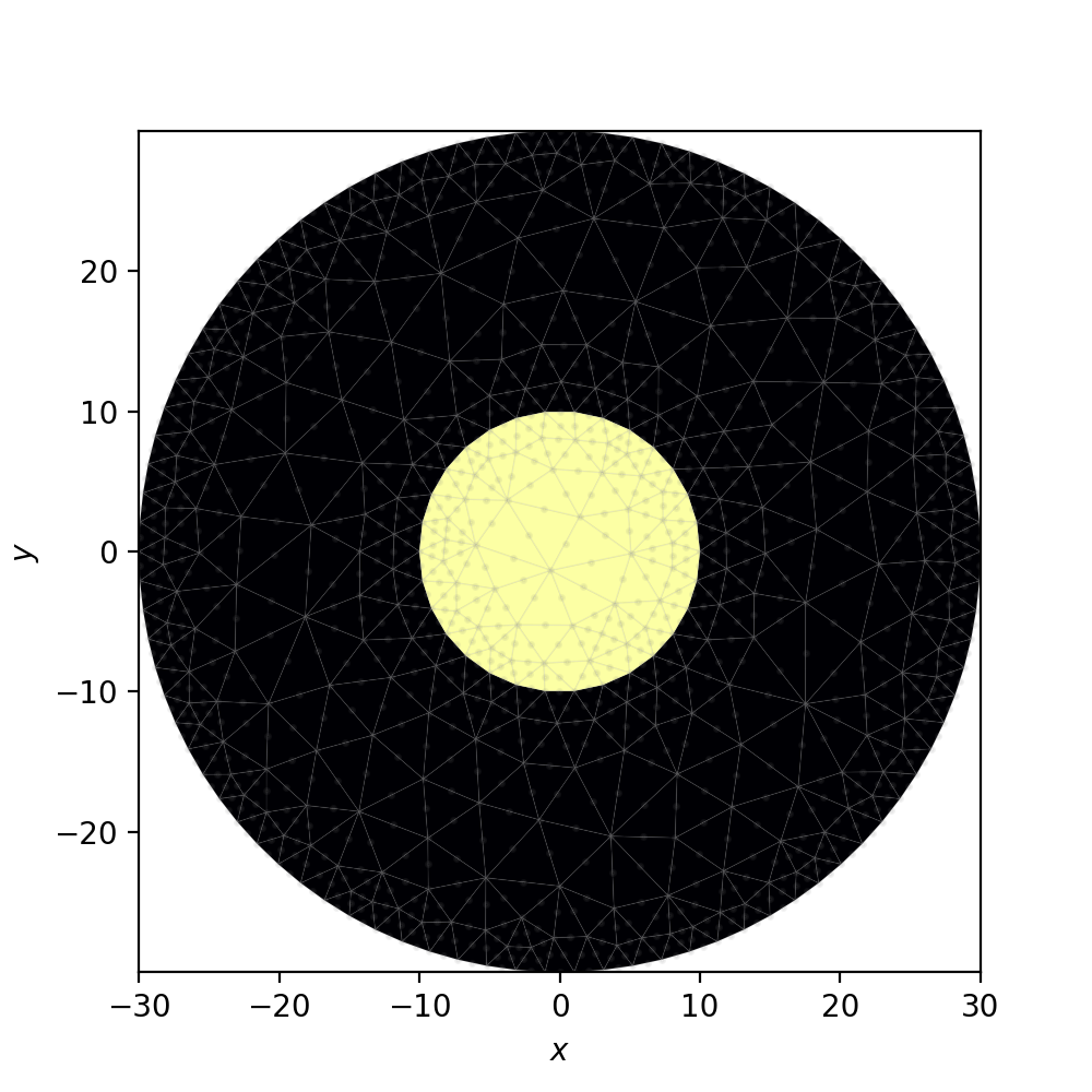
Note that core comes after clad, ensuring that the region inside the core cylinder has index ncore instead of nclad. Let’s check our work by making a mesh and plotting.

mesh = fiber.make_mesh()
fiber.plot_mesh(mesh=mesh)

(Source code, png, hires.png, pdf)

Because fiber cross section doesn’t change with \(z\), running a characterization using cbeam.propagator isn’t necessary. However, we may still use cbeam to look at the modes, using solve_at().

from cbeam.propagator import Propagator
wavelength = 1.55 # um
Nmax = 10 # solve for 10 modes
prop = Propagator(wavelength,fiber,Nmax)
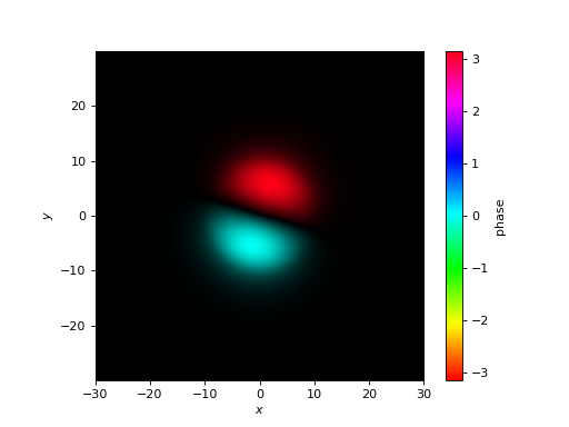
effective_indices, modes = prop.solve_at(0) # could solve at any z value too
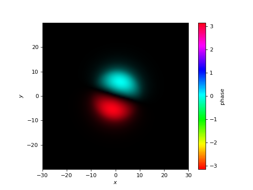
prop.plot_cfield(modes[1],res=0.5) # look at LP_11

(Source code, png, hires.png, pdf)

1.2. tapered square fiber

For a slightly more involved example, we’ll make a rectangular fiber which tapers in one axis with \(z\), loosely inspired by edge couplers and tapers for multimode interferometers. We’ll use the BoxPipe class to construct this tapered fiber.

length = 10000 # um
xw_core = lambda z: 10 * (1+2*z/length) # triples in thickness over length
yw_core = 10 # fixed height

rect_core = waveguide.BoxPipe(ncore,"core",xw_core,yw_core)

xw_clad = lambda z: 30 * (1+2*z/length)

# cladding will just be a bigger core
rect_clad = waveguide.BoxPipe(nclad,"clad",xw_clad,3*yw_core)

(Source code)

We’ll also set target mesh sizes inside the core and cladding, then create the Waveguide.

rect_clad.mesh_size = 3. # target size of triangles in cladding (but not core)
rect_core.mesh_size = 1. # target size in core

rect_fiber = waveguide.Waveguide([rect_clad,rect_core])

(Source code)

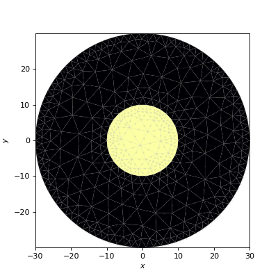
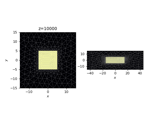
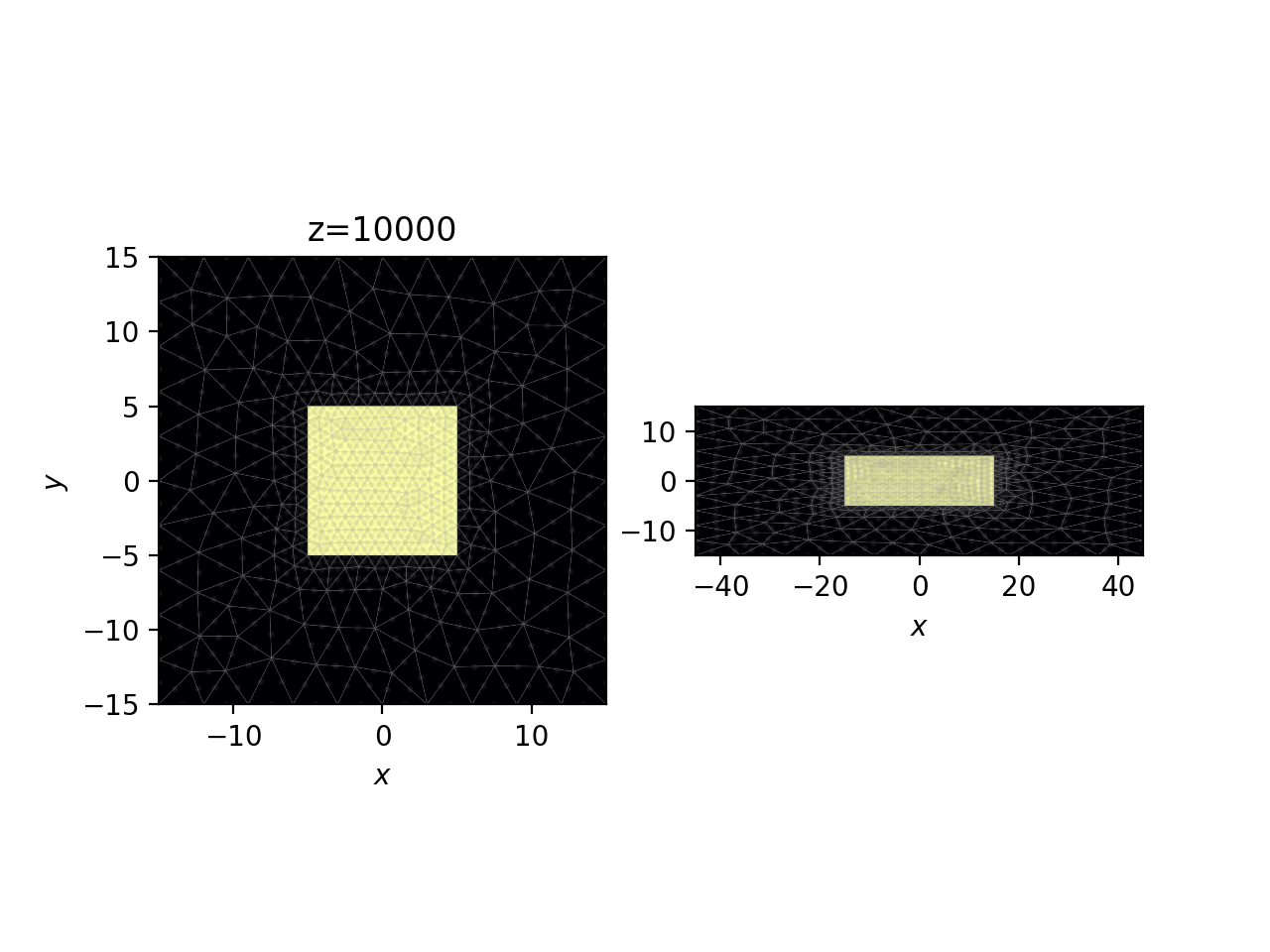
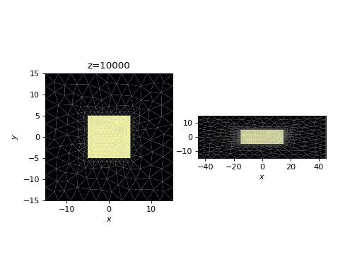
Now, we’ll plot meshes at different \(z\) values.

fig,axs = plt.subplots(1,2)
rect_fiber.plot_mesh(z=0,ax=axs[0])
rect_fiber.plot_mesh(z=length,ax=axs[1])
axs[0].set_title("z=0")
axs[0].set_title("z="+str(length))
plt.show()

(Source code, png, hires.png, pdf)

Note the following:

1. A transformation rule did not have to be specified. The Waveguide class performs the transformation automatically.

2. The transformation in this case increases triangle skewness. This can lead to lower accuracy; in cases of extreme skewness, you should consider breaking up the waveguide in \(z\), or checking convergence properties by increasing the mesh resolution.

Moving on, let’s solve for the effective indices and modes of this waveguide as a function of \(z\).

# solve for top 6 modes in terms of effective index
rect_prop = Propagator(wavelength,rect_fiber,6)

rect_tag = "tapered_box"

# comment/uncomment below as necessary
rect_prop.compute_neffs(0,length,save=True,tag=rect_tag)
# rect_prop.load(rect_tag)

# if you wanted a more careful computation of the modes, you could also use
# rect_prop.compute_modes()

(Source code)

Now, we’ll take a look at the effective indices of the modes.

rect_prop.plot_neffs()

(Source code, png, hires.png, pdf)

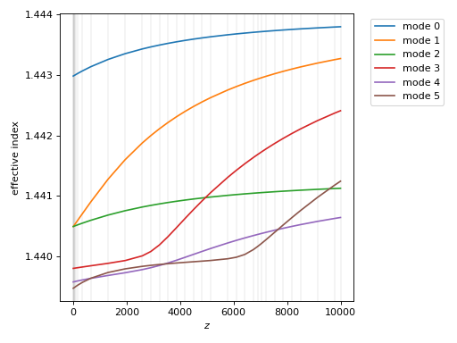
Vertical lines indicate the \(z\) values used during the calculation. The fundamental mode has the highest effective index, and is the blue curve in the above. The next two modes (orange and green), which are \(LP_{11}\)-like, start out as degenerate in eigenvalue, as expected; the degeneracy splits with \(z\). All modes after mode 2 are initially cladding modes - you can tell because the effective index starts lower than lowest index in our waveguide. But as the waveguide widens, these modes becomes bound, and their eigenvalues cross in complicated ways.

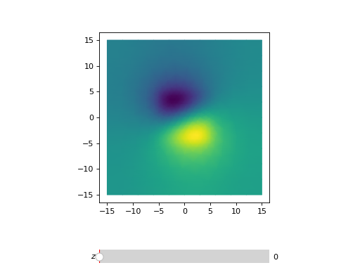
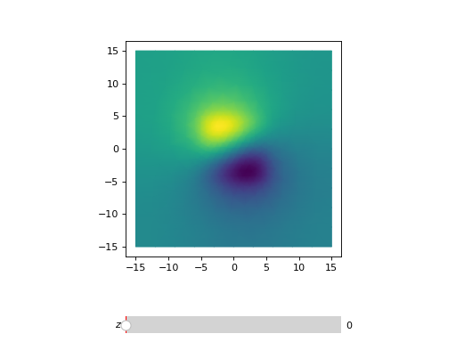
Finally, we will view the \(z\)-dependent eigenmodes of the waveguide using plot_waveguide_mode(). If you run the below on your own you should get a slider which can be used to set the \(z\) value. Unfortunately, the slider rendered below is not interactive.

# plot eigenmode 2
rect_prop.plot_waveguide_mode(2)

(Source code, png, hires.png, pdf)