1. 3-port photonic lantern#
1.1. Making the waveguide#
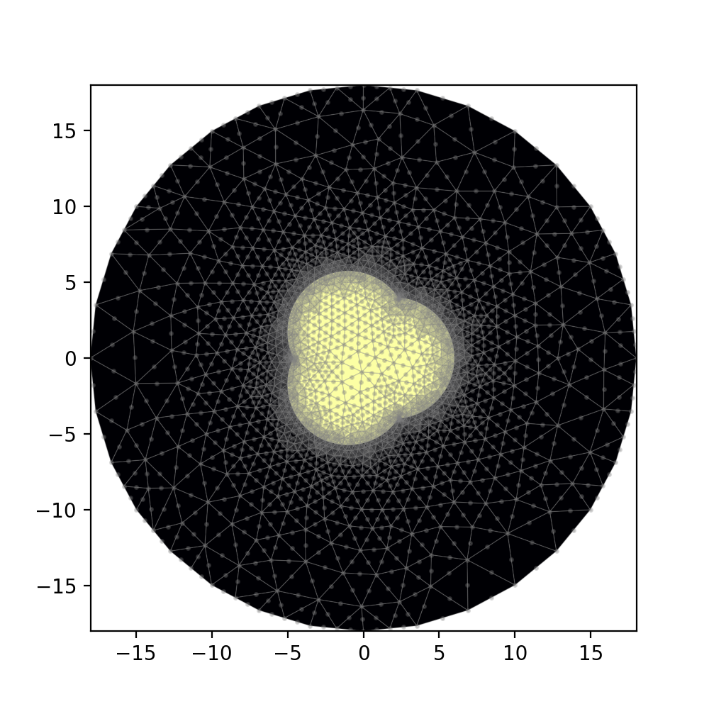
Below we use the waveguide module to make a 3-port photonic lantern, formed by tapering down a bundle of 3 single-mode fibers embedded inside a low-index capillary often referred to as the “jacket”. The small end of such a device typically has a flower-shaped core (which is really formed from the cladding material of the single-mode fibers) that can be approximated by 3 overlapping circles, each corresponding to one of the fibers in the bundle.
First, here are our parameters.
from wavesolve import waveguide
import numpy as np
import matplotlib.pyplot as plt

## params
ncore = 1.444+5e-3 # core index
nclad = 1.444 # cladding index

rcore = 4. # radius of circles composing flower-shaped core
rclad = 18. # cladding radius (outer simulation boundary)
res = 64 # resolution for boundaries

core_offset = 2. # radial offset of circles forming the core
Now, let’s make 3 Circle objects, which will be boolean unioned to formed the irregular core. Note that Circle objects, and more generally the Prim2D (“2D primitive”) class, which is used to represent all closed 2D shapes and which forms the basis of Waveguide geometry, is initialized as
primitive = Prim2D(n,label)
where n is the refractive index inside the shape, and label is a bookkeeping name to be assigned to the shape.
All Prim2D objects also have a function make_points(), which is used to generate the boundary of the represented shape.
Below I construct the irregular core, the cladding, and the Waveguide.
offsetsx = [1,np.cos(2*np.pi/3),np.cos(4*np.pi/3)]
offsetsy = [0,np.sin(2*np.pi/3),np.sin(4*np.pi/3)]
offsets = np.array([offsetsx,offsetsy]).T * core_offset
# make overlapping circular claddings
core_circs = []
for o in offsets:
circ = waveguide.Circle(ncore,"") # label doesnt matter since we will combine these
circ.make_points(rcore,res,o) # make points corresponding to radius rcore, resolution res, centerpoint o
core_circs.append(circ)
# combine the Circles using Prim2DUnion, a type of Prim2D
core = waveguide.Prim2DUnion(core_circs,"core")
clad = waveguide.Circle(nclad,"clad")
clad.make_points(rclad,int(res/2)) # lower resolution for the outer boundary
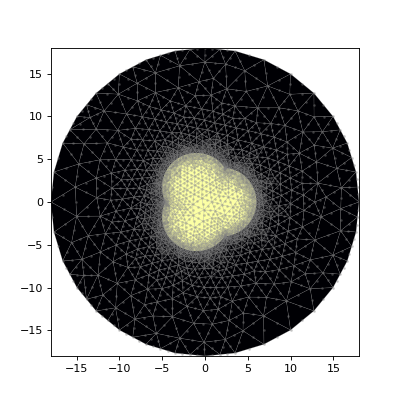
PL3 = waveguide.Waveguide([clad,core])
PL3.plot_mesh()
(Source code, png, hires.png, pdf)
1.2. Solving#
Now let’s solve for the eigenmodes.
import matplotlib.pyplot as plt
from wavesolve.FEsolver import solve_waveguide, plot_scalar_field, count_modes
IOR_dict = PL3.assign_IOR()
mesh = PL3.make_mesh()
wl = 1.55
# not sure how many modes there will be so we'll use the
# optional Nmax arg to get the first 10 modes
_w,_v = solve_waveguide(mesh,wl,IOR_dict,Nmax=10)
# get number of modes
Nmodes = count_modes(_w,wl,IOR_dict)
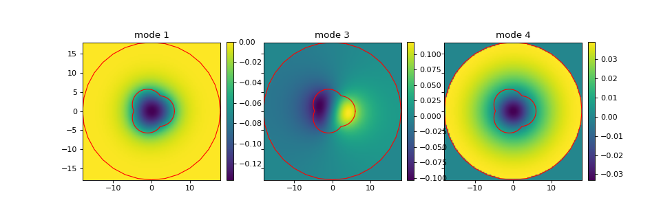
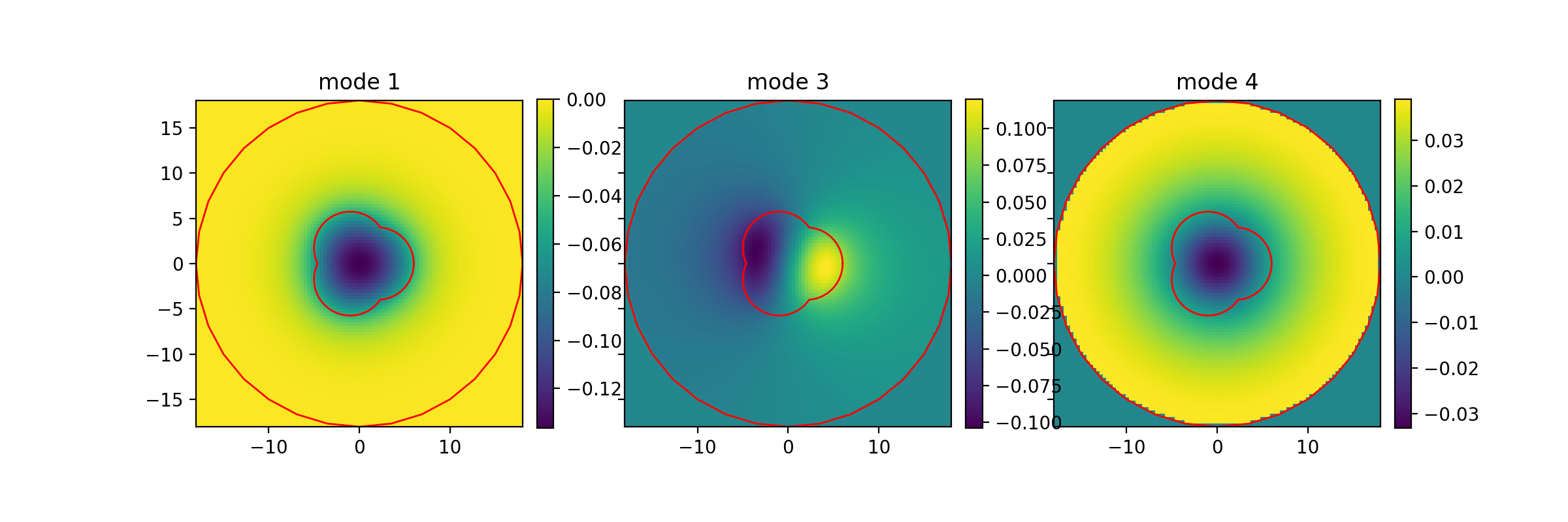
fig,axs = plt.subplots(1,3,sharex=True,sharey=True,figsize=(12,4))
plot_scalar_field(mesh,_v[0],show_mesh=False,ax=axs[0])
plot_scalar_field(mesh,_v[Nmodes-1],show_mesh=False,ax=axs[1])
plot_scalar_field(mesh,_v[Nmodes],show_mesh=False,ax=axs[2])
for ax in axs:
PL3.plot_boundaries(ax) # show the waveguide boundary
axs[0].set_title("mode 1")
axs[1].set_title("mode "+str(Nmodes))
axs[2].set_title("mode "+str(Nmodes+1))
plt.show()
(Source code, png, hires.png, pdf)

The number of guided modes is again 3. For the above, I’m also showing the waveguide boundaries with Waveguide.plot_boundaries(). The last plot shows a typical spurious/cladding mode, which is non-zero in the cladding.