3. Hollow core photonic crystal fiber

Hollow core fibers guide light in a lower-index region (e.g. in air), which is surrounded by a higher index substrate with periodic structure. In this case, guidance is provided by the so-called photonic bandgap, which is analogous to the electronic gap between Brillouin zones in crystals. The eigenmodes of such a waveguide are trickier to find because they have lower effective index, and so effective index information alone is insufficient to identify spurious modes. In these cases, we search for modes by specifying an upper bound on effective index for the guided mode.

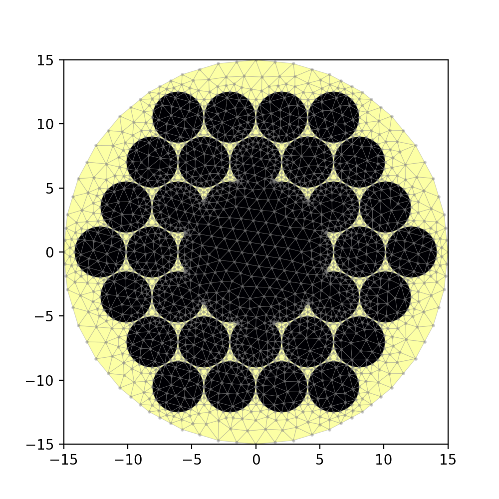
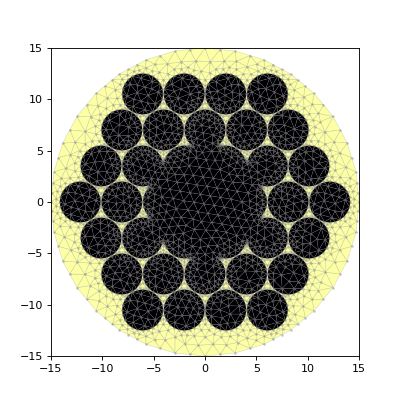
Below is an example. First we’ll make the mesh, which must be order 1 since this waveguide has high index contrast. The specs are loosely based off the images I found of NKT hollow core fibers.

from wavesolve.waveguide import PhotonicBandgapFiber

void_radius = 11.5/2    # hollow core radius
hole_radius = 2.        # radius for air holes in cladding
clad_radius = 15.       # outer boundary radius
nclad = 1.444           # cladding index
hole_separation = 4.05  # separation between air holes
hole_res = 24           # air hole boundary resolution
clad_res = 32           # outer boundary (cladding) resolution

hollow_PCF = PhotonicBandgapFiber(void_radius,hole_radius,clad_radius,nclad,hole_separation,hole_res,clad_res,hole_mesh_size=1.0,clad_mesh_size=2.0)
m = hollow_PCF.make_mesh(order=1)
hollow_PCF.plot_mesh(m)

(Source code, png, hires.png, pdf)

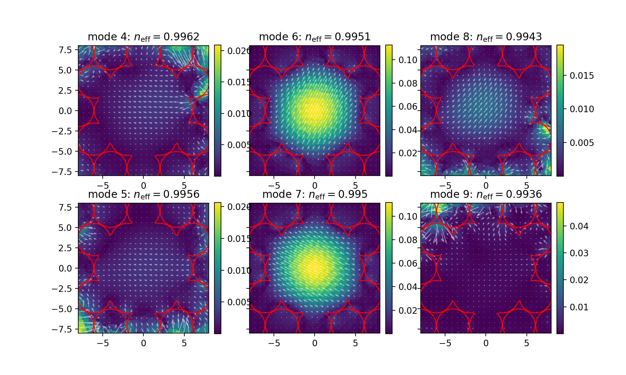
Next, let’s solve. The voids in this fiber have index 1, so I will search for modes with the largest indices at and below 1, using the optional target_neff argument in solve_waveguide_vec().

from wavesolve.FEsolver import get_eff_index,plot_vector_field,solve_waveguide_vec
import matplotlib.pyplot as plt, numpy as np

IOR_dict = hollow_PCF.assign_IOR()
wl = 1.65

ws,vs = solve_waveguide_vec(m,wl,IOR_dict,target_neff=1.0,Nmax=10)
ne = get_eff_index(wl,ws)

fig,axs = plt.subplots(2,3,sharey=True,figsize=(10,6))
for j,ax in enumerate(axs.T.flatten()):
    i = j+3
    plot_vector_field(m,vs[i],ax=ax,bounds=(-8,8,-8,8))
    hollow_PCF.plot_boundaries(ax)
    ax.set_title("mode "+str(i+1)+r": $n_{\rm eff}=$"+str(round(np.real(ne[i]),4)))

plt.show()

(Source code, png, hires.png, pdf)

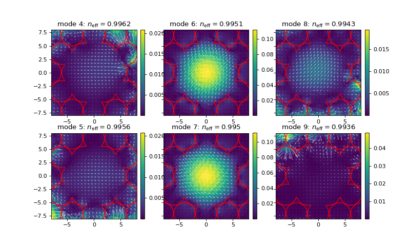
After solving for the first 10 modes, I find that modes 6 and 7 are physical, with effective index \(\approx 0.995\).