Quickstart

1. waveguide basics

Waveguides are defined as classes. There are several pre-defined classes, and users may define their own which inherit from a base Waveguide class. The full documentation is here.

Waveguide objects have one ultimate purpose: they create finite-element meshes, through

mesh = Waveguide.make_mesh()

Eigenmodes are computed on this mesh. Waveguide objects also have auxiliary plotting functions. Using the pre-defined CircularFiber class, which represents a circular step-index optical fiber, as an example:

from wavesolve.waveguide import CircularFiber

#params
rcore = 5               # core radius, assumed um
rclad = 15              # outer radius of simulation boundary, um
ncore = 1.444+8.8e-3    # core refractive index
nclad = 1.444           # cladding refractive index
core_res = 64           # number of line segments used to refine the core-cladding boundary
clad_res = 64           # number of line segments for outer clad boundary

# make waveguide
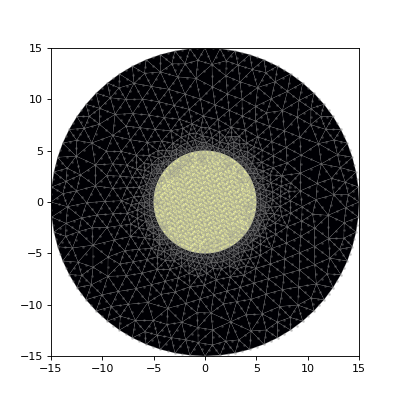
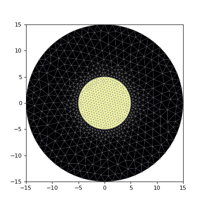
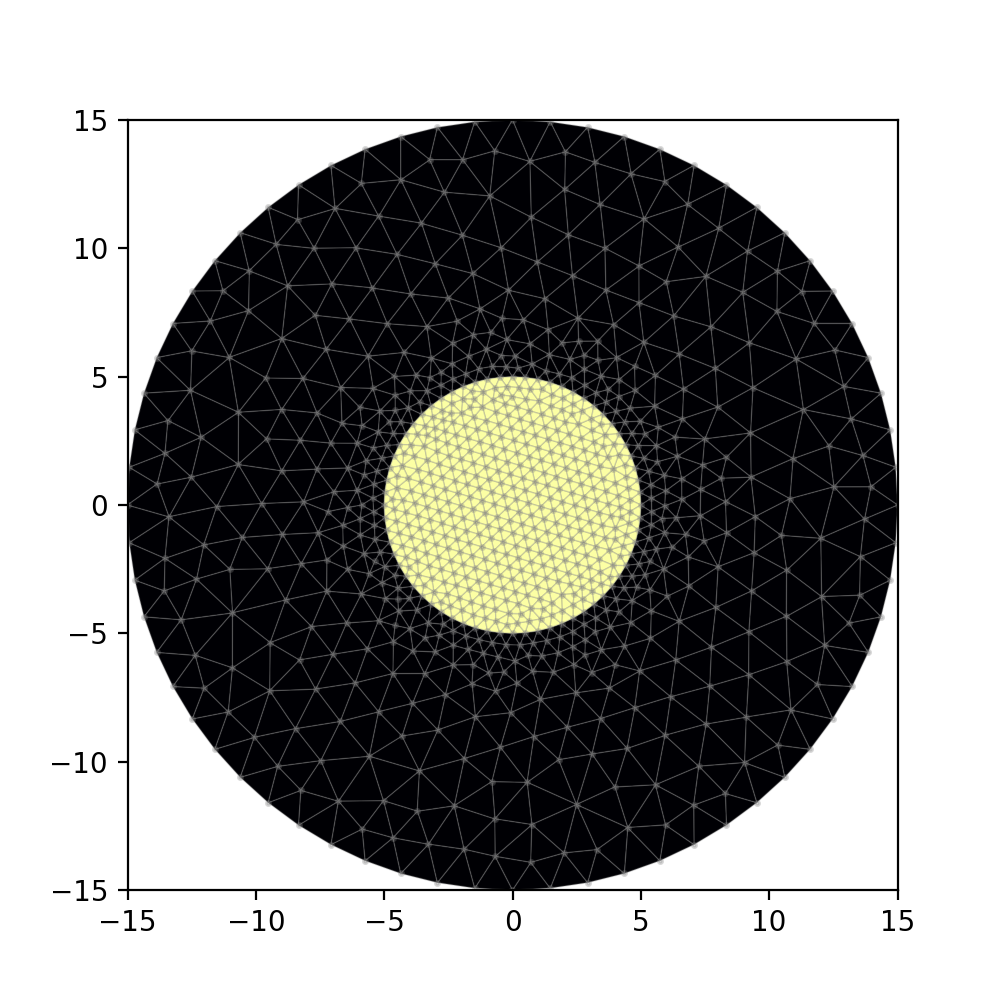
fiber = CircularFiber(rcore,rclad,ncore,nclad,core_res,clad_res,core_mesh_size=0.5)

# make a plot mesh
mesh = fiber.make_mesh()
fiber.plot_mesh(mesh=mesh)

(Source code, png, hires.png, pdf)

More generally, Waveguide objects are constructed from a list of 2D primitives (waveguide.Prim2D), which contain both geometry and refractive index information; examples include Circle and Rectangle. For instance, the CircularFiber above is essentially the same as Waveguide([clad,core]), where clad and core are the cladding and core Circle objects, respectively. Later items in the list overwrite earlier items in refractive index.

Every Waveguide also comes with the function assign_IOR(), which creates a Python dictionary that maps mesh triangles to refractive index values. This is how refractive index information is passed to the mode solver. Let’s make the dictionary for fiber.

IOR_dict = fiber.assign_IOR()

(Source code)

2. FEsolver basics - scalar

This module takes meshes generated by waveguide and solves the corresponding generalized eigenvalue problem to get the waveguide eigenvectors. Each element in an eigenvector corresponds to an electric field amplitude at a point in the finite element mesh.

Given a mesh, we solve for the scalar eigenmodes using

eigvals, eigvecs = FEsolver.solve_waveguide(mesh,wl,IOR_dict)

where the arguments are as follows:

1. mesh : the finite element mesh generated by Waveguide.make_mesh()

2. wl : the target wavelength, in the same units as for mesh

3. IOR_dict : a dictionary which assigns groups of triangles in mesh to their refractive index value, e.g. the output of Waveguide.assign_IOR()

The return values are

1. eigvals : the array of eigenvalues

2. eigvecs : the matrix of eigenvectors; each row is an eigenvector.

I use the CircularFiber from earlier an an example:

from wavesolve.FEsolver import solve_waveguide

wl = 1.55 # um
eigvals, eigvecs = solve_waveguide(mesh,wl,IOR_dict)

(Source code)

The eigenvalues correspond to \(\beta^2\) where \(\beta\) is the mode propagation constant. Eigenvalues can be converted to effective refractive indices using FEsolver.get_eff_index(wl,eigval).

To view the eigenvectors, we can use

FEsolver.plot_scalar_field(mesh,field,ax=None,bounds=None)

which has the arguments

1. mesh : the finite element mesh

2. field : the scalar field (e.g. eigenvector) to be plotted

3. ax : (optional) a matplotlib axis to plot on; if None, an axis will be made

4. bounds : 4-element array [xmin,xmax,ymin,ymax], setting plot boundary. If None, use the mesh boundary

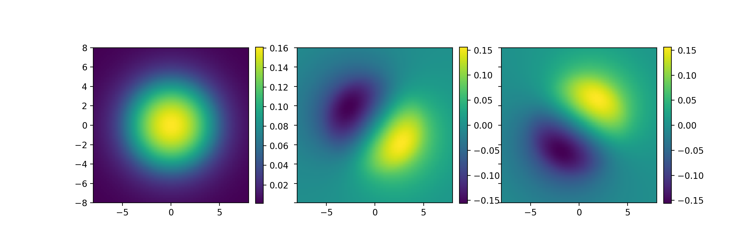
Below I plot the first 3 modes from above.

from wavesolve.FEsolver import plot_scalar_field
import matplotlib.pyplot as plt

fig,axs = plt.subplots(1,3,sharey=True,figsize=(12,4))
for i,ax in enumerate(axs):
    ax.set_aspect('equal')
    plot_scalar_field(mesh,eigvecs[i],ax=ax,bounds=(-8,8,-8,8))
plt.show()

(Source code, png, hires.png, pdf)

These are the LP₀₁ and LP₁₁ modes; the rest are spurious cladding modes. For waveguides with weak index contrast, the number of non-spurious guided modes may be computed using count_modes:

from wavesolve.FEsolver import count_modes
num_modes = count_modes(eigvals,wl,IOR_dict)
print("number of guided modes: ",num_modes)

(Source code)

This should give the output

number of guided modes:  3

To evaluate the field amplitude at an arbitrary point, use

field_amp = FEsolver.evaluate(point,field,mesh)

where point is a \(2\times 1\) array containing the \(x\) and \(y\) coordinates of interest, field is the field vector (e.g. an eigenmode), and mesh is the finite element mesh on which field was computed.

3. FEsolver basics - vector

Vectorial mode solving is a requirement for high-index-contrast waveguides. To solve for the vector modes, we can use

eigvals, eigvecs = FEsolver.solve_waveguide_vec(mesh,wl,IOR_dict)

The syntax is similar to the scalar solve_waveguide(). However, there is an important difference. The vectorial solver is only implemented for meshes of linear triangular elements (order 1) whereas the default mesh generation and scalar solver assume order 2. We need to specify this when generating the mesh: mesh = Waveguide.make_mesh(order=1).

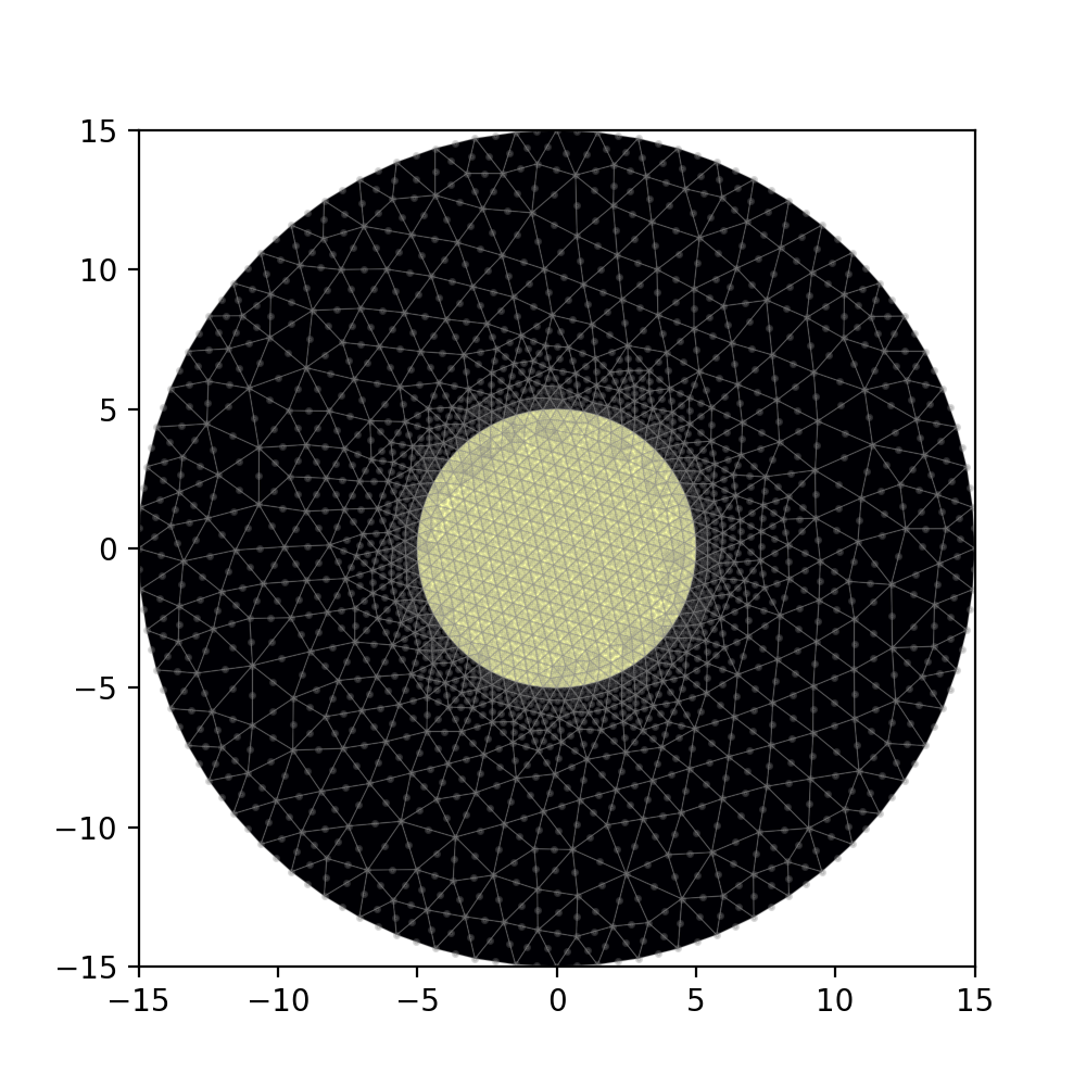
As an example, I will solve for the vector modes of the same 3-mode step index circular fiber. First, let’s generate an order 1 mesh.

mesh_ord1 = fiber.make_mesh(order=1)

# plot the mesh
fiber.plot_mesh(mesh=mesh_ord1)

(Source code, png, hires.png, pdf)

The triangles in this mesh have only 3 points, corresponding to vertices (order 2 triangular elements also have edge midpoints).

Next, we’ll use solve_waveguide_vec() to get the modes. Since the fiber supports 3 LP modes, we expect 6 vector modes. To confirm this, let’s solve for the 7 modes with the highest eigenvalues, using the Nmax optional argument.

from wavesolve.FEsolver import solve_waveguide_vec
# default Nmax is 6
eigvals_ord1,eigvecs_ord1 = solve_waveguide_vec(mesh_ord1,wl,IOR_dict,Nmax=7)

(Source code)

To plot, we can use plot_vector_field(mesh,field), which has similar syntax to plot_scalar_field(). First we’ll plot the guided modes.

from wavesolve.FEsolver import plot_vector_field

fig,axs = plt.subplots(2,3,sharex=True,sharey=True,figsize=(12,8))
for i,ax in enumerate(axs.flatten()):
    plot_vector_field(mesh_ord1,eigvecs_ord1[i],ax=ax,bounds=(-8,8,-8,8))
plt.show()

(Source code, png, hires.png, pdf)

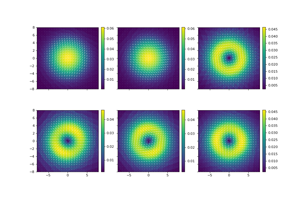
In this case, we pass in premade matplotlib axes, and the function plots the transverse field component. The first two modes are the HE₁₁ modes. The next four modes are linear combinations of the TE₀₁, TM₀₁, and HE₂₁ modes, which have the same effective index.

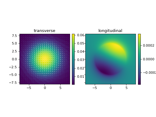
Without providing an axis, the default plotting behavior is to show both the transverse and longitudinal components. E.g. for the first HE₁₁ mode:

plot_vector_field(mesh_ord1,eigvecs_ord1[0],bounds=(-8,8,-8,8))

(Source code, png, hires.png, pdf)

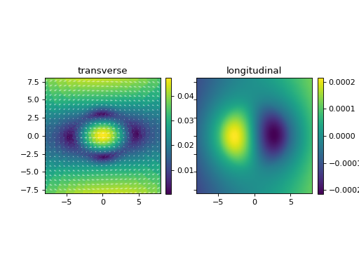
The amplitude of the longitudinal field is quite small, which expected considering the weak index contrast of this waveguide. Let’s also look at mode 7, which I claimed was spurious.

plot_vector_field(mesh_ord1,eigvecs_ord1[6],bounds=(-8,8,-8,8))

(Source code, png, hires.png, pdf)

Warning

In the vectorial case, distinguishing between spurious and non-spurious modes becomes more difficult. In general, FEsolver.count_modes will not work for vector modes. It will only work when index contrast is weak (such as in this fiber example). In other cases, use the eye test!

Finally, to evaluate a vector-valued field, use the same function as in the scalar case:

field_amp_xy, field_amp_z = FEsolver.evaluate(point,field,mesh)

where field_amp_xy is the vector-valued transverse component of field at point, and field_amp_z is the scalar longitudinal component.